|
a free and open toolkit for 2d/3d seismic data analysis |
|
kogeo seismic toolkit |


|
Contact:
|
|
Phone (home): +49 - 40 - 2780 7890 Phone (office): +49 - 40 - 42838 5234 Fax: +49 - 40 - 42838 7081 E-Mail: konerding@geowiss.uni-hamburg.de |
|
Features |
|
The data editing (processing) functions in kogeo can be accessed from the ‘Data->Data editing‘ menu:
They’re only available if the current session contains data. If you choose a menu item, the corresponding dialog will appear. All of them are organized in a similar way; pressing the ‘start’ button actually starts the editing process. When working on 3d data, editing function are only available if the data is organized in a project database. After the editing process, 3d data is saved as a temporary data file. This one can be added to the database as a new version when the result is satisfactory or deleted by choosing the ‘Data->Close active data’ menu item.
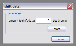
Time shift:
The data is shifted up or down in time, this is only useful to correct 2d data misfits.
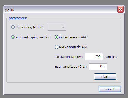
Fixed gain, AGC:
Applies fixed or automatic gain to your data. There’re two versions of AGC: instantaneous and RMS amplitude AGC.
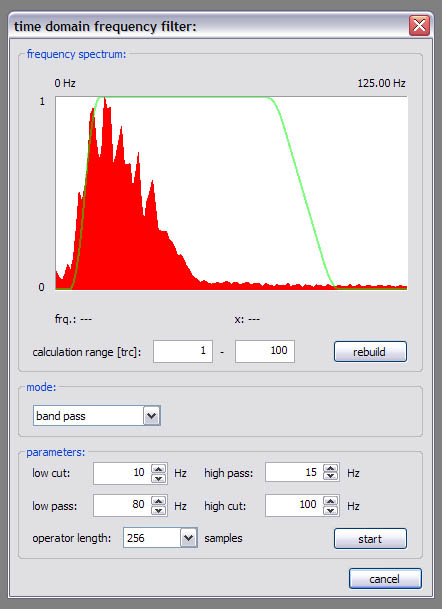
Time domain frequency filter:
This performs frequency filtering in the time domain. You can choose an operator length in the ‘parameters’ section and different filter form modes in the ‘mode’ section of the dialog window. When the dialog window is created, a frequency spectrum is calculated over a given range of traces, it can be recreated by pressing the ‘rebuild’ button. The spectrum is scaled linearly with the dominant frequency always assigned to a value of 1. According to the filter form mode, you’ll need to specify frequencies in the ‘parameters’ section of the dialog window, the resulting filter form is shown in green on the frequency spectrum.
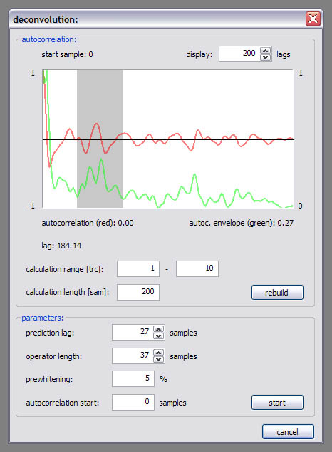
Predictive deconvolution:
In the upper part of the dialog window a stacked autocorrelation function is displayed (red line); it’s envelope function is shown in green (in my opinion energy maxima are easier to see on this one, that’s why). You can specify the trace range, calculation length and display length, the starting point for the autocorrelation calculation has to be entered in the ‘parameters’ section on the bottom of the dialog window. Use the ‘rebuild’ button, if you’ve changed one of the settings. The parameters for the filter operator design are given in the ‘parameters’ section (‘prediction lag’ and ‘operator length’), the grey bar in the autocorrelation window is drawn according to these settings. You can specify a ‘prewhitening’ percentage, like it’s described in the literature (e.g. Yilmaz).
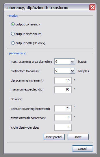
Coherency, dip/azimuth transform:
Coherency and dip/azimuth can be calculated together when working in 3d mode or must be calculated separately otherwise. They are estimated by measuring and (weighted) averaging of semblance along constructed ‘reflectors’ of different dips and azimuth values. Specify a ‘static azimuth correction’ to account for true inline directions and an x-bin size/y-bin size unequal to 1 if the inline and crossline distances are not the same. Dip/azimuth datasets require a specially formatted colorbar to be displayed properly. You can find one in the collection of colorbars in the download section. Mail me if there’re further questions!
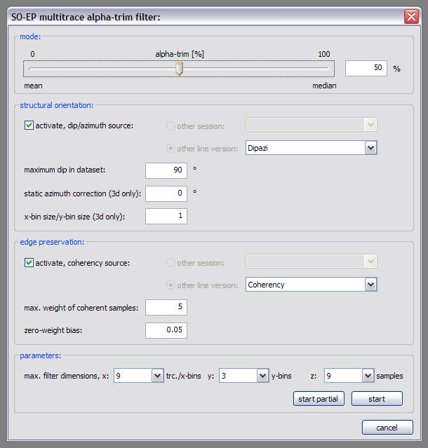
SO-EP multitrace alpha-trim filter:
In it’s basic version, the multitrace alpha-trim filter performs smoothing by calculating the mean, median or a mixture of both according to the alpha-trim setting. The calculation is performed in a window around every sample; it’s dimensions are specified in the ‘parameters’ section of the dialog window. SO-EP means ‘structurally oriented’ and ‘edge preserving’, two options you can activate to improve the filtering results. For SO filtering you need to specify a kogeo-dip/azimuth dataset and it’s calculation parameters. EP filtering is accomplished by taking the coherency structure of the considered sub-volume into account. The samples are weighted according to their coherence and the coherency-path between individual samples. Choose a ‘max. weight for coherent samples’ (sample weight when coherency equals 1.0) and a ‘zero-weight bias’ (samples with lower coherence than the given value are not weighted).
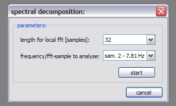
Spectral decomposition:
In spectral decomposition local fft’s of a given length are performed (centered around the respective sample) to retrieve local frequency spectra. The intensity of the adjusted frequency is assigned then as the new value for the considered sample.
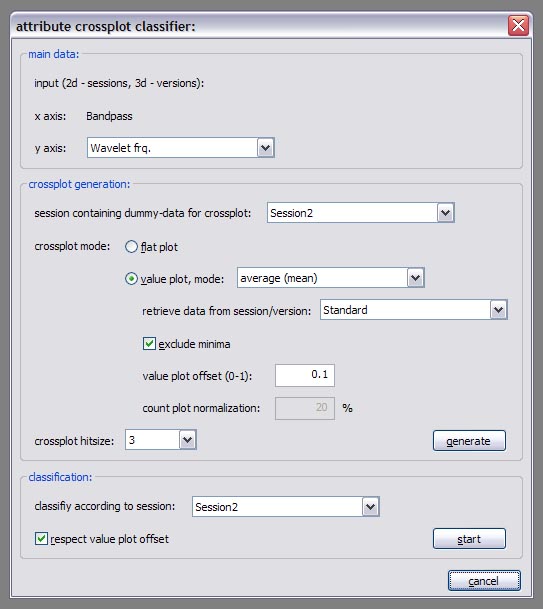
Attribute crossplot classifier:
With this functions attribute crossplots can be created and data can be classified according to them. To create a crossplot, first specify a secondary data source (representing the y-axis of the resulting crossplot). In the ‘crossplot generation’ section, you can setup where (‘session containing dummy data for crossplot’) and how (’crossplot mode’) the crossplot will be generated. If you choose to build a ‘value plot’, you’ll also have to specify a way how multiple hits on the crossplot are treated (or if they’re just counted, when ‘count-plot’ is chosen). Hits on the crossplot will be assigned to values retrieved from the source specified under ‘retrieve data from session/version’; samples with a value of -1.0 will be ignored, when ‘exclude minima’ is activated. An additional ‘value plot offset’ can be specified to separate low values and areas of no hits. In count-plots the results will be scaled according to the ‘count plot normalization’ percentage. If the ‘crossplot hitsize’ parameter is higher than one, a hit on the crossplot will occupy more than just one sample, but a quadratic area of the given edge length. When data is to be classified according to an attribute crossplot, the crossplot source must be specified. If the crossplot was created with a ‘value plot offset’, activate the ‘respect value plot offset’ option. The offset is taken from the field in the ‘crossplot generation’ section.
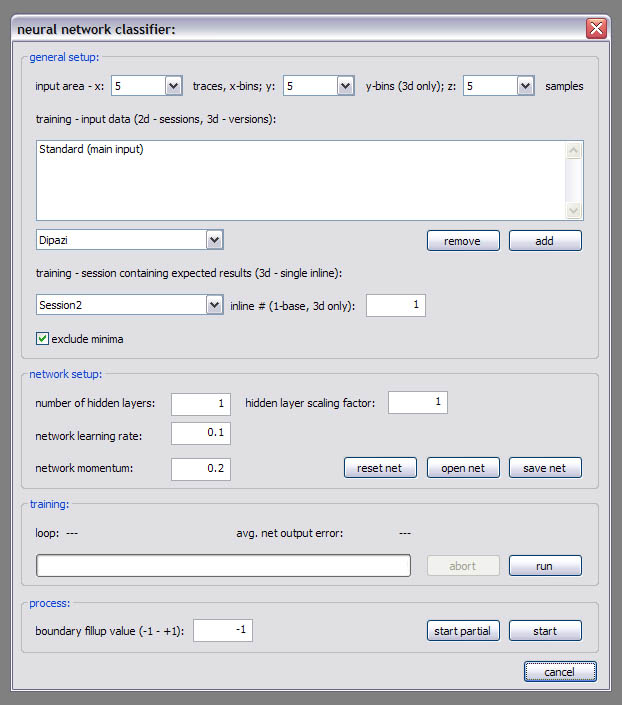
Neural network classifier:
The ‘Neural network classifier’ generates meta-attributes by the classification of a neural network. The network is of the multi-layer perceptron type and it’s training is achieved using the back-propagation algorithm. A trained network can be saved and used later on again to classify data. Don’t panic when a ‘...training information will be lost’ message appears before you have actually trained your network; this is due to the necessary physical reconstruction of the network when some of the parameters are changed. Under ‘general setup’ you can choose several sets of input data that feed the network and one dataset that is used to compare the values predicted by the network during training (‘session containing expected results’). Input data of all input data sets is retrieved from the ‘input area’, which is centered around the positions of samples in the reference dataset. If the ‘exclude minima’ option is activated, reference samples with a value of -1 are ignored during the training. The ‘network setup’ section contains information about how the network is physically constructed. The size of the input layer is given by the size of the input area multiplied by the number of input data sets. A ‘number of hidden layers’ (layers between the input layer and the output layer) is created according to the value given, a ’hidden layer scaling’ of 1 means that they’ll have the same size like the input layer. The size of the output layer is 1. The ‘run’ button in the ‘training session’ will start the network training, in the dialog that appears you’ll be asked to specify a depth range and a number of training loops. You might also activate the logging function which will store the training results in a .dbf table. They can be plotted in Excel then or something else. While the training is running, the progress is shown and if it’s successful you should see a (probably slowly) decreasing ‘avg. net output error’. The training can be stopped and restarted at any time. In the ‘process’ section you can start the neural network classification process itself. The ‘boundary fillup value’ is necessary, because areas that overlap the dataset’s extent can’t be properly processed; they’re filled with the respective value instead. Resample:
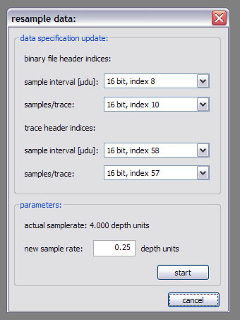
The resampling function works only on 2d data and performs quadratic interpolation to resample each trace with the new sample interval given in the lower part of the dialog window. The header values are updated according to the settings in the upper part of the dialog window. |

Read more about... |
|
...data editing |

|
You‘re visitor no.: |
|
Home |
|
About kogeo |
|
Features |
|
Download |
|
Building instructions |
|
Guestbook |
|
Home |
|
About kogeo |
|
Features |
|
Download |
|
Building instructions |
|
Guestbook |